Profiling Python ⋆ Mark McDonnell

Memory Management

Before we dive into the techniques and tools available for profiling Python applications, we should first understand a little bit about its memory model as this can help us to understand what it is we’re seeing in relation to memory consumption.

Python manages memory using reference counting semantics. What this means is, every time an object is referenced, either by a variable assignment or similar, the counter for that object is incremented. Once an object is not referenced anymore its memory is deallocated (its counter is decremented every time a reference is removed, until it reaches zero). But as long as there is a reference (somewhere in the program), then the object will not be deallocated (as the internal counter will be greater than zero).

Now this can cause problems when dealing with cyclical references, so that’s something to be aware of when investigating memory leaks and other memory related concerns.

Note: for lots of details of how Python allocates memory, I highly recommend this presentation.

Types of Profiling

There are a couple of approaches available to us for monitoring performance…

Timers: useful for benchmarking, as well as comparing before and after fixes.
Profilers: useful for high-level verification.

Tools Matrix

	Pros	Cons
timer (decorator)	- Simple, quick and easy.	- Requires code change. - Adds latency & skews results.
timeit module	- Calculate repeat averages. - Doesn’t require code change.	- More complicated API.
profiler module	- Granular CPU by file. - Can be run from terminal.	- More complicated results. - Read docs to understand.
line_profiler	- Granular line-by-line CPU.	- Slow. - Not built-in package. - Requires code change.
memory_profiler	- Clear and easy results.	- Slow † - Not built-in package. - † additional packages help.
tracemalloc	- Built-in memory package.	- Requires code change. - More complicated API.
pyflame	- Visualise problem area easily. - Details CPU and Memory	- Requires Linux. - Most complex to setup.

Analysis Steps

Regardless of the tool you use for analysis, a general rule of thumb is to:

Identify a bottleneck at a high-level

For example, you might notice a long running function call.

Reduce the operations

Look at time spent, or number of calls, and figure out an alternative approach.
Look at the number of memory allocations, figure out an alternative approach.

Drill down

Use a tool that gives you data at a lower-level.

Think about more performant algorithms or data structures.
There may also be simpler solutions.
Take a pragmatic look at your code.

Base Example

Let’s begin with a simple program written using Python 3…

def get_number():
    for i in range(10000000):
        yield i


def expensive_function():
    for n in get_number():
        r = n ^ n ^ n
    return f"some result! {r}"


print(expensive_function())

Note: I’m currently using Python version 3.6.3

Running this program can take ~1.8 seconds and returns the value:

some result! 9999999

Timer

We can use a simple decorator to time the length of our expensive_function call…

from time import time
from functools import wraps


def timefn(fn):
    """Simple timer decorator."""
    @wraps(fn)
    def measure_time(*args, **kwargs):
        t1 = time()
        result = fn(*args, **kwargs)
        t2 = time()
        print(f"@timefn: {fn.__name__} took {str(t2 - t1)} seconds")
        return result
    return measure_time

The problem with this approach is that the decorator results in additional latency. Meaning the program takes slightly longer to complete. Not a lot, but if you’re after precision then this can skew the results (which is a common theme when benchmarking or profiling).

Built-in module: timeit

The built-in timeit module is another simple way of benchmarking the time it takes for a function to execute. Simply import the module and call its interface.

import timeit
…
result = timeit.timeit(expensive_function, number=1)  # one repetition
print(result)

Note: you can tweak the number param to determine how many repetitions it’ll run.

Along with the timeit method, there is a repeat method that returns a set of averages across the number of repeated code executions.

result = timeit.repeat(expensive_function, number=1, repeat=5)

In this case result would contain something like:

[1.7263835030025803, 1.7080924350011628, 1.6802870190003887, 1.6736655100103235, 1.7003267239924753]

Note: according to the Python documentation when utilising the repeat method you should only be interested in the min() because…

“In a typical case, the lowest value gives a lower bound for how fast your machine can run the given code snippet; higher values in the result vector are typically not caused by variability in Python’s speed, but by other processes interfering with your timing accuracy”.

Finally, there is also a command line version you can utilise:
python -m timeit

Built-in module: profiler

There are two flavours of profiler, a pure Python version (import profile) and a C extension version (import cProfile) which is preferred, as the former is remarkably slower.

For example, the C profile took ~3 seconds to complete, whereas the Python version took over a minute.

Note: if using cProfile you would execute: cProfile.run("expensive_function()") otherwise you would execute profile.run("expensive_function()").

You should see something like the following displayed after executing your program:

         10000005 function calls in 3.132 seconds

   Ordered by: standard name

   ncalls  tottime  percall  cumtime  percall filename:lineno(function)
 10000001    1.042    0.000    1.042    0.000 3_profile.py:4(get_number)
        1    2.090    2.090    3.132    3.132 3_profile.py:9(expensive_function)
        1    0.000    0.000    3.132    3.132 <string>:1(<module>)
        1    0.000    0.000    3.132    3.132 {built-in method builtins.exec}
        1    0.000    0.000    0.000    0.000 {method 'disable' of '_lsprof.Profiler' objects}

So from these results we can see:

There were a total of 10000005 function calls.
The get_number function was called the most (10000001).
Every other function in the total recorded, were called just the once.
The expensive_function took a total of 2.090 seconds (exc. sub function calls).
The cumulative time (cumtime) is the tottime plus sub function calls.

Note: when there are two numbers in the first column (for example 3/1), it means that the function recursed. The second value is the number of primitive calls and the former is the total number of calls. Note that when the function does not recurse, these two values are the same, and only the single figure is printed.

Instead of printing the results you can pass the run method a second argument which is a filename you want to store the results in. Once there you can use the pstats.Stats module to carry out some post-processing on those results.

Finally, there is also a command line version you can utilise:
python -m cProfile [-o output_file] [-s sort_order] <your_script.py>

Line Profiler

The Line Profiler option gives much more granular detail than the built-in profile module, but it is an external package and so needs to be installed:

pip install line_profiler

Once installed you can write a decorator to wrap the functionality and make it easier for applying to specific functions you want to profile (as demonstrated below).

from line_profiler import LineProfiler


def do_profile(follow=None):
    if not follow:
        follow = []

    def inner(func):
        def profiled_func(*args, **kwargs):
            try:
                profiler = LineProfiler()
                profiler.add_function(func)
                for f in follow:
                    profiler.add_function(f)
                profiler.enable_by_count()
                return func(*args, **kwargs)
            finally:
                profiler.print_stats()
        return profiled_func
    return inner


def get_number():
    for i in range(10000000):
        yield i


@do_profile(follow=[get_number])
def expensive_function():
    for n in get_number():
        r = n ^ n ^ n
    return f"some result! {r}"


print(expensive_function())

We can see the result of executing this program below…

Timer unit: 1e-06 s

Total time: 7.59566 s
File: 4_line_profile.py
Function: get_number at line 23

Line #      Hits         Time  Per Hit   % Time  Line Contents
==============================================================
    23                                           def get_number():
    24  10000001      3924533      0.4     51.7      for i in range(10000000):
    25  10000000      3671129      0.4     48.3          yield i

Total time: 27.477 s
File: 4_line_profile.py
Function: expensive_function at line 28

Line #      Hits         Time  Per Hit   % Time  Line Contents
==============================================================
    28                                           @do_profile(follow=[get_number])
    29                                           def expensive_function():
    30  10000001     22122124      2.2     80.5      for n in get_number():
    31  10000000      5354911      0.5     19.5          r = n ^ n ^ n
    32         1            3      3.0      0.0      return f"some result! {r}"

some result! 9999999

Note: the Line Profiler is pretty slow (~35s) in comparison to the cProfiler (~4s)

The Line Profiler will typically only analyse the function being decorated. In order for it to include sub function calls, you’ll need to specify them (hence the decorator allows you to provide a list of functions and in there we’ve specified the get_number function).

The order in which you list the sub functions to ‘follow’ doesn’t matter, as the results will always display (top to bottom) the deepest nested sub function to the top level function (so we can see that get_number is nested inside of expensive_function and so it is top of the output).

From these results we can get a line-by-line breakdown of how long (in percentages) each function took to complete. So expensive_function spent ~20% of its time calculating a value to assign to the variable r, and the remaining 80% was spent calculating a value to assign to the variable n (which was the call out to the get_number function).

As for get_number, it was approximately 50/50 for time between looping the range(10000000) and yield’ing a value back to the caller context (i.e. expensive_function).

Finally, there is also a command line version you can utilise:

kernprof -l [-v view_results] <your_script.py>

If you omit the -l flag, then you can view the results at a later time using:

python -m line_profiler <your_script.py>.lprof

Basic Memory Profiler

There is a module called memory_profiler which is very simple to use, although with the example code we’ve been using it was so painfully slow it was pretty much unusable (I gave up after 5 minutes of waiting). So, because of that issue, I’ll demonstrate a simpler example.

But first you need to install the module:

pip install memory_profiler
pip install psutil  # recommended to help speed up the reporting time

Now you can import the decorator, and apply that to our new ‘slow’ function:

from memory_profiler import profile

@profile
def expensive_memory_allocations():
    a = [1] * (10 ** 6)
    b = [2] * (2 * 10 ** 7)
    del b
    return a

print(len(expensive_memory_allocations()))

When you run this program, you’ll see a memory breakdown similar to the following:

Line #    Mem usage    Increment   Line Contents
================================================
    35     27.8 MiB      0.0 MiB   @profile
    36                             def beep():
    37     35.4 MiB      7.6 MiB       a = [1] * (10 ** 6)
    38    188.0 MiB    152.6 MiB       b = [2] * (2 * 10 ** 7)
    39     35.4 MiB   -152.6 MiB       del b
    40     35.4 MiB      0.0 MiB       return a

The second column “Mem usage” indicates the memory consumption for the Python interpreter after that line was executed. The third column “Increment” indicates the difference in increased memory compared to the previous line that was executed. So you can see, for example, when we delete the b variable we are able to reclaim the memory it was holding on to.

Tracemalloc

There is another basic memory profiler that provides similar features called tracemalloc but this particular tool is part of the standard library in Python so it might be preferable to the external library memory_profiler (shown earlier).

import tracemalloc


def get_number():
    for i in range(10000000):
        yield i


def expensive_function():
    for n in get_number():
        r = n ^ n ^ n
    return f"some result! {r}"


tracemalloc.start()

print(expensive_function())

snapshot = tracemalloc.take_snapshot()
top_stats = snapshot.statistics("lineno")

print("[ Top 10 ]")
for stat in top_stats[:10]:
    print(stat)

The output from this example is as follows:

$ time python tracemalloc_example.py

some result! 9999999

[ Top 10 ]
tracemalloc_example.py:17: size=106 B, count=2, average=53 B

Note: You might also consider Pympler or ObjGraph for tracking memory usage & object refs.

PyFlame (Flame Graphs)

Flame graphs are a visualization of profiled software (stack traces), allowing the most frequent code-paths to be identified quickly and accurately. Flame graphs allows hot code-paths to be identified quickly.

PyFlame is an effective tool (written in C++) for generating flame graph data, which can help you to understand the CPU and memory characteristics of your services. In some cases it can report more accurate results than those provided by the built-in Python modules.

For more details on the design decisions behind PyFlame and the shortcomings of the other built-in options, then I would recommend reading this article.

PyFlame only works with Linux operating systems and so in order to profile our code (if you’re using macOS like I am), then we’ll have to utilise Docker to help us. Below is a Dockerfile you can use as a basic starting point to try out PyFlame.

Note: we also require FlameGraph in order to generate the flame graphs.

FROM python:3.6.3

WORKDIR /pyflame

# Install dependencies required to ‘build’ PyFlame
RUN apt-get update -y
RUN apt-get install -y git autoconf automake autotools-dev g++ pkg-config python-dev python3-dev libtool make

# Build PyFlame
RUN git clone https://github.com/uber/pyflame.git && \
    cd pyflame && ./autogen.sh && ./configure && make

WORKDIR /flamegraph

RUN git clone https://github.com/brendangregg/FlameGraph

COPY 7_pyflame.py /app/app.py

WORKDIR /app

CMD /pyflame/pyflame/src/pyflame -o prof.txt -t python app.py &&\
    /flamegraph/FlameGraph/flamegraph.pl ./prof.txt

In order to build and run this Dockerfile, you’ll need to execute the following code…

docker build -t pyflame .

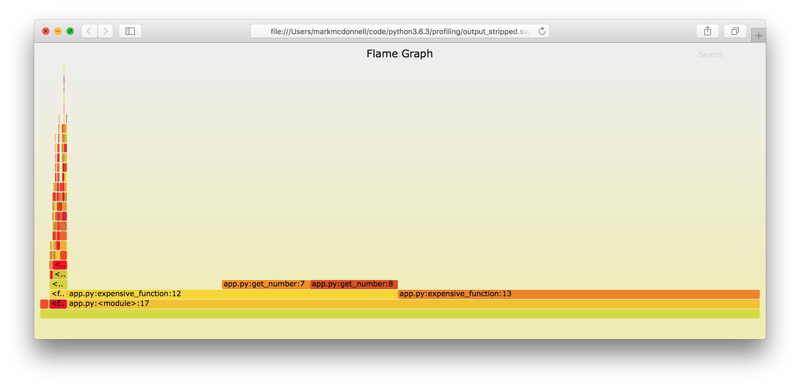
docker run --privileged pyflame > output.svg && tail -n+2 output.svg > output_stripped.svg

Note: our application sends data to stdout (e.g. some result! 9999999) and so this ends up at the top of our output.svg file. This means we need to remove it. We could either modify the application code or you could do what I’ve done and strip it after the file is created by using the tail command and redirecting the stripped output to a new file: output_stripped.svg.

If we now open output_stripped.svg we should see the following interactive flame graph.

Conclusion

That’s our tour of various tools for profiling your Python code. I’ll follow this article up with a Go based one in the very near future. But if you’re interested in further reading then the following blog posts from rushter.com are worth a look: