Algorithms in Python
In this post I’ll be demonstrating a few common algorithms using the Python language. I’m only covering a very small subset of popular algorithms because otherwise this would become a long and diluted list.
Instead I’m going to focus specifically on algorithms that I find useful and are important to know and understand:
- Sorting
- Searching
But before we get into it... time for some self-promotion 🙊
Three out of the four ‘search’ algorithms listed above will be implemented around a graph data struture. Graphs appear everywhere in life. For example, your Facebook list of friends, mutual friends, and extended friends (i.e. friends of your friends who you don’t know) is a perfect example of a ‘graph’.
Graphs can also be ‘weighted’, so they can indicate that a relationship between two nodes within the graph are possibly stronger than another connection, and is typically used in road maps for determining the quickest path to a particular node (we’ll come back to this later when reviewing Dijkstra’s Algorithm).
Merge Sort
Given an unsorted list of integers, the merge sort algorithm enables us to sort the list.
- Best:
Ω(n log(n)) - Average:
O(n log(n)) - Worst:
O(n log(n))
The algorithm can be broken down into the following pseudo-steps:
- Recursively split given list into two partitions.
- Divide the list until reaching its smallest partition.
- Recursively merge each pair of partitions (repeat till reconstructed list).
That short list actually defines two distinct processes: a ‘break up into partitions’ step followed by a ‘merge’ step. The merge pseudo-steps could be further broken down to look something like the following:
- To merge two partitions we iterate over each of them.
- Compare elements from both partitions (left and right).
- Append smaller element to new ‘results’ (i.e. sorted) list.
- After comparing the elements, increment index for winning partition.
The above merge steps process is carried out against each recursively sorted set of partitions, and is done until we reach a final ‘sorted’ list.
Below is an implementation of this sorting algorithm:
def merge(left, right):
    left_index, right_index = 0, 0
    result = []

    while left_index < len(left) and right_index < len(right):
        if left[left_index] < right[right_index]:
            result.append(left[left_index])
            left_index += 1
        else:
            result.append(right[right_index])
            right_index += 1

    result += left[left_index:]
    result += right[right_index:]

    return result


def merge_sort(collection):
    if len(collection) <= 1:
        print('collection is <= 1\n')
        return collection

    middle = len(collection) // 2
    left = collection[:middle]
    right = collection[middle:]

    left = merge_sort(left)
    right = merge_sort(right)

    return merge(left, right)

collection = [10, 5, 2, 3, 7, 0, 9, 12]

result = merge_sort(collection)

print(f'merge sort of {collection} result: {result}\n\n')
Quick Sort
Given an unsorted list of integers, the merge sort algorithm enables us to sort the list.
- Best:
Ω(n log(n)) - Average:
O(n log(n)) - Worst:
O(n^2)
The algorithm can be broken down into the following pseudo-steps:
- Pick a ‘pivot’ (e.g. random index from the list).
- Iterate the collection twice, creating two new lists.
- Create a list consisting of elements less than pivot.
- Create a list consisting of elements greater than pivot.
- function return value is
fn(less) + pivot + fn(greater).
Note: notice the ’less’ and ‘greater’ lists are passed recursively back through the quick sort function.
Below is an implementation of this sorting algorithm:
from random import randrange

collection = [10, 5, 2, 3, 7, 0, 9, 12]

def quicksort(collection):
    if len(collection) < 2:
        return collection
    else:
        random = randrange(0, len(collection))
        pivot = collection.pop(random)

        less = [i for i in collection if i <= pivot]
        greater = [i for i in collection if i > pivot]

        return quicksort(less) + [pivot] + quicksort(greater)

cloned_collection = collection.copy()  # avoid mutation

result = quicksort(cloned_collection)

print(f'quick sort of {collection} result: {result}\n\n')
Difference between Merge and Quick sort
Both merge sort and quick sort are ‘divide and conquer’ algorithms, e.g. they divide a problem up into two and then process the individual partitions, and will keep dividing up the problem for as a long as it can.
So when considering which you should use (i.e. which is better?) you’ll find merge sort is more performant because its particular implementation is more efficient with the operations it carries out.
Specifically, the difference between merge sort and quick sort is that with quick sort you’ll loop over the collection twice in order to create two partitions, but remember that doing so doesn’t mean the partitions are sorted.
These quick sort partitions are not sorted until the recursive calls end up with a small enough partition (length of 1) where the left and right partitions can be analyzed, joined and therefore considered ‘sorted’.
Compare that to merge sort which recursively creates multiple partitions (all the way down to the smallest possible partition) before it then recursively rolls back up the execution stack and attempts to sort each of the partitions along the way.
Additionally, with a merge sort it’s possible to parallelize the data over multiple processes, while quick sort requires data to be processed within a single process.
This means that quick sort has potentially more operations to be carried out than merge sort, and therefore has a greater time complexity. Although quick sort can offer better ‘space’ complexity (worst case: O(log(n))) compared to merge sort (worst case: O(n)).
All that said, the implementation of the algorithms can be tweaked as needed to produce better or worst performance. For example, quick sort could be modified to use another algorithm called intro sort which is a mix of quick sort, insertion sort, and heapsort, that’s worst-case O(n log(n)) but retains the speed of quick sort in most cases.
Radix Search?
Another searching algorithm that I see crop up in discussions every now and then is ‘radix search’. The way it works is to loop over your data structure twice and (if we’re dealing with integers) for the first iteration you’ll ‘bucket’ the elements by their 1’s digit, followed by another iteration to bucket the elements by their 10’s digit.
So with a collection like 25, 17, 85, 94, 32, 79, after the first iteration we would have created ’numbered’ buckets that looked something like the following:
1: <empty>
2: 32
3: <empty>
4: 94
5: 25, 85
6: <empty>
7: 17
8: <empty>
9: 79
If we remove the empty buckets it means we’ll end up with a partially sorted list of 32, 94, 25, 85, 17, 79. Now for the second iteration we re-bucket by the 10’s, so this means we end up with:
1: 17
2: 25
3: 32
4: <empty>
5: <empty>
6: <empty>
7: 79
8: 85
9: 94
Again if we remove the empty buckets we’ll find we now have a fully sorted list: 17, 25, 32, 79, 85, 94.
It’s an interesting algorithm but ultimately is quite limited and so other sorting algorithms like merge/quick sort are generally preferred. Some constraints to be aware of are is that it’s generally less efficient than other comparison sorting algorithms.
Radix sort is also targeted at integers, fixed size strings, floating points and <, > or lexicographic order comparison predicates.
Binary Search
The most popular algorithm (by far) for searching a value in a sorted list is ‘binary search’. The reason for its popularity is that it provides logarithmic performance (on average) for access, search, insertion and deletion operations.
- Average:
O(log(n)) - Worst:
O(n)
The algorithm can be broken down into the following pseudo-steps:
- define ‘start’ and ’end’ positions (usually length of list).
- locate middle of list.
- stop searching if correct value found.
- if value is greater: change end position to the middle index.
- if value is smaller: change start position to the middle index.
- repeat above steps until value is found.
What this ultimately achieves is shortening the search ‘window’ of items by half each time (that’s the logarithmic part). So if you have a list of 1000 elements, then we can say it’ll take a maximum of ten operations to find the number you’re looking for (that’s: log 2(10) == 2^10 == 1024).
That’s outstanding.
Below is an implementation of this popular search algorithm:
def binary_search(collection, item):
    start = 0
    stop = len(collection) - 1

    while start <= stop:
        middle = round((start + stop) / 2)
        guess = collection[middle]

        if guess == item:
            return middle
        if guess > item:
            stop = middle - 1
        else:
            start = middle + 1

    return None

collection = [1, 3, 5, 7, 9, 11, 13, 15, 17, 19, 20, 21]

result = binary_search(collection, 9)

print(f'the value was found at index {result}\n\n')  # index 4
Note: you could swap
round((start + stop) / 2)for(start + stop) // 2which uses Python’s//floor division operator, but I typically opt for the clarity of using the explicitroundfunction.
Breadth First Search
A BFS (breadth first search) is an algorithm that searches a data structure from either a root node or some arbitrary starting point. It does this by exploring all the neighbouring nodes, before moving onto other connected nodes.
The following graph represents a group of people. Some people know each other (e.g. both Alice and Bob know each other), where as other people don’t (e.g. Dave knows Ethan, but Ethan knows no one else in this group).
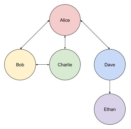
We’ll use the BFS (breadth first search) algorithm to locate ‘Ethan’.
The time complexity of this algorithm will be, at worst, O(V+E).
Note: in the case of dealing with a graph,
V= vertex (a node in the graph) andE= edge (the line between nodes), the worst case scenario will mean we have to explore every edge and node.
The algorithm can be broken down into the following pseudo-steps:
- Pick a starting point in the data structure.
- Track nodes to process (e.g. a queue).
- While the queue has content:
- Take a node from the queue.
- If the node has been searched already, then skip it.
- If not searched, check if it’s a match, otherwise update queue.
- Queue should be updated with that node’s adjacent nodes.
- If match is found, then exit the queue loop.
Below is our example implementation of the BFS algorithm:
import random
from collections import deque

graph = {'alice': ['bob', 'charlie', 'dave'],
         'bob': ['alice', 'charlie'],
         'charlie': ['alice', 'bob'],
         'dave': ['alice', 'ethan']}

def search(starting_point, name):
    print(f'starting point: {starting_point}')

    queue = deque()
    queue += graph[starting_point]  # add starting_point's neighbours
    print(f'queue: {queue}')

    searched = []

    while queue:
        person = queue.popleft()
        print(f'person: {person}')

        if person not in searched:
            if person == name:
                print(f'found a match: {person}')
                return True
            else:
                queue += graph[person]  # add this item's neighbours
                print(f'queue updated: {queue}')
                searched.append(person)
        else:
            print(f'skipping {person} as they have already been searched')

    return False

starting_point = random.choice(list(graph.keys()))
search(starting_point, 'ethan')
Note: an alternative implementation might use Python’s
setdata structure to avoid having to filter already searched people.
Let’s take a look at the first run of this program:
starting point: dave
queue: deque(['alice', 'ethan'])
person: alice
queue updated: deque(['ethan', 'bob', 'charlie', 'dave'])
person: ethan
found a match: ethan
From that output we can see that we started very conveniently at the ‘Dave’ node. Dave’s adjacent nodes are Alice and Ethan. Due to the order of the nodes in the queue we attempt to process Alice next. Then we check the next node (Ethan) and find what we’re looking for.
Now consider a second run which has a different starting point (notice the difference in the number of operations):
starting point: charlie
queue: deque(['alice', 'bob'])
person: alice
queue updated: deque(['bob', 'bob', 'charlie', 'dave'])
person: bob
queue updated: deque(['bob', 'charlie', 'dave', 'alice', 'charlie'])
person: bob
person: charlie
queue updated: deque(['dave', 'alice', 'charlie', 'alice', 'bob'])
person: dave
queue updated: deque(['alice', 'charlie', 'alice', 'bob', 'alice', 'ethan'])
person: alice
skipping alice as they have already been searched
person: charlie
skipping charlie as they have already been searched
person: alice
skipping alice as they have already been searched
person: bob
skipping bob as they have already been searched
person: alice
skipping alice as they have already been searched
person: ethan
found a match: ethan
Note: I’ve used a dict to represent a graph, which helped to make the code simpler to understand. A different data structure (e.g. a directed tree) would require a different implementation of the algorithm. Remember, the basic premise is to search a graph node’s adjacent fields, and then their adjacent nodes.
Depth First Search
The following image shows a tree structure that represents various people…
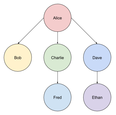
A DFS (depth first search) is an algorithm that searches a data structure (such as a tree, or a graph) from its root node. It searches downwards through each child node until there are no more children.
We’ll use the DFS (depth first search) algorithm to locate the node ‘Ethan’.
Using our example tree structure (above) we would start with Alice, then check the first child Bob. Bob has no children so we would move onto Charlie. Charlie has a single child Fred so we would check him next. Fred has no children so we start back up at Dave. Finally, we check the child of Dave which is Ethan.
Notice how if don’t find a match for what we’re looking for, then we backtrack up to the top of the tree and start again at the root node’s next child node.
The time complexity of this algorithm will be, at worst, O(V+E) (as noted with Breath First Search, this means we could end up hitting every single node and edge in the data struture).
Note: this example uses a traditional tree data structure instead of a graph to represent the underlying data to be searched.
The algorithm can be broken down into the following pseudo-steps:
- Start at the root node.
- Check first child to see if it’s a match.
- If not a match, check that child’s children.
- Keep checking the children until a match is found.
- If no children are a match, then start from next highest node.
Below is our example implementation of the DFS algorithm:
class Tree(object):
    def __init__(self, name='root', children=None):
        self.name = name
        self.children = []

        if children is not None:
            for child in children:
                self.add_child(child)

    def __repr__(self):
        return self.name

    def add_child(self, node):
        assert isinstance(node, Tree)
        self.children.append(node)


tree = Tree('Alice', [Tree('Bob'),
                      Tree('Charlie', [Tree('Fred')]),
                      Tree('Dave', [Tree('Ethan')])])


def search_tree(tree, node):
    print(f'current tree: {tree}')

    if tree.name == node:
        print(f'found node: {node} in {tree}')
        return tree

    for child in tree.children:
        print(f'current child: {child}')

        if child.name == node:
            print(f'found node: {node} in {child}')
            return child

        if child.children:
            print(f'attempt searching {child} for {node}')
            match = search_tree(child, node)

            if match:
                print(f'returning the match: {match}')
                return match

result = search_tree(tree, 'Ethan')

print(f'result: {result}')
Note: in our example we use a simple tree data structure to represent the data to be searched. Our implementation is designed to work with that structure. So, for example, if we had multiple children per node (left and right child nodes), then we would need to account for the backtrack to the relevant child right node near the top of the tree.
Let’s take a look at the output of this program:
current tree: Alice
current child: Bob
current child: Charlie
attempt searching Charlie for Ethan
current tree: Charlie
current child: Fred
current child: Dave
attempt searching Dave for Ethan
current tree: Dave
current child: Ethan
found node: Ethan in Ethan
returning the match: Ethan
result: Ethan
So from this output we can see we started at Alice, and first checked Bob but because Bob has no children we moved back up to Charlie. From Charlie we go down to Fred but as there’s no more children we move back up to Dave. Finally we check Dave’s children to find Ethan.
When to choose BFS vs DFS?
Generally BFS is better when dealing with relationships across fields, where as DFS is better suited to tree hierarchies.
That said, below is a short list of things to consider when opting for either a BFS or DFS:
Note: the data strutures used (including the implementation of your algorithm) can also contribute to your decision.
- If you know the result is not far from the root: BFS.
- If result(s) are located deep in the structure then: DFS.
- If the depth of the structure is very deep, then in some cases: BFS.
- If the width of the structure is very wide, then memory consumption could mean: DFS.
Ultimately, it all depends.
Searching an unsorted collection?
If you have an unsorted collection, then your only option for searching is a linear time complexity O(n). To improve that performance we would need to first sort the collection so we could use a binary search on it.
Another potential option is to run a linear search across multiple CPU cores so you’re effectively parallelizing the processing. It’s still O(n) linear time complexity, but the perceived time would be shorter (depending on the restructuring of the collection split chunks).
Dijkstra’s Algorithm
The Dijkstra algorithm tells you the quickest path from A to B within a weighted graph.
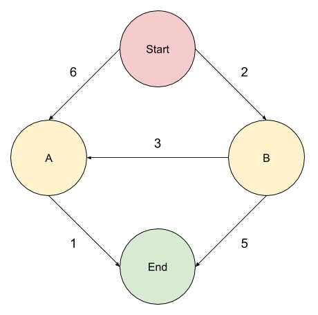
In the above graph we have a few options:
- Start > A > End (Cost: 7)
- Start > B > End (Cost: 7)
- Start > B > A > End (Cost: 6)
Note: as you can see, the route that visually looks longer is actually quicker when considering the weighted nature of the graph.
The time complexity of this algorithm will be, at worst, O(V+E) (as noted with Breath First Search and Depth First Search, this means we could end up hitting every single node and edge in the data struture).
The algorithm can be broken down into the following pseudo-steps (it’s important to note that in this implementation we calculate the route in reverse):
- Identify the lowest cost node in our graph.
- Acquire the adjacent nodes.
- Update costs for each node while accounting for surrounding nodes.
- Track the processed nodes.
- Check for new lowest cost node.
These steps are very specific to our graph, so if your data structure is different, then the implementation of the algorithm will need to change to reflect those differences. Regardless this should be a nice introduction to the fundamental properties of the algorithm.
Without further ado, below is an example implementation of the Dijkstra’s algorithm:
graph = {
    'start': {
        'a': 6,
        'b': 2
    },
    'a': {
        'end': 1
    },
    'b': {
        'a': 3,
        'end': 5
    },
    'end': {}
}

costs = {
    'a': 6,
    'b': 2,
    'end': float('inf')  # set to infinity until we know the cost to reach
}

parents = {
    'a': 'start',
    'b': 'start',
    'end': None  # doesn't have one yet until we choose either 'a' or 'b'
}

processed = []
route = []

def find_lowest_cost_node(costs):
    lowest_cost = float('inf')
    lowest_cost_node = None

    for node in costs:
        cost = costs[node]

        if cost < lowest_cost and node not in processed:
            lowest_cost = cost
            lowest_cost_node = node

    return lowest_cost_node

def find_fastest_path():
    node = find_lowest_cost_node(costs)

    while node is not None:
        cost = costs[node]
        neighbours = graph[node]

        for n in neighbours.keys():
            new_cost = cost + neighbours[n]

            if costs[n] > new_cost:
                costs[n] = new_cost
                parents[n] = node
        processed.append(node)
        node = find_lowest_cost_node(costs)

def display_route(node=None):
    if not node:
        route.append('end')
        display_route(parents['end'])
    elif node == 'start':
        route.append(node)
        reverse_route = list(reversed(route))
        print('Fastest Route: ' + ' -> '.join(reverse_route))
    else:
        route.append(node)
        display_route(parents[node])

find_fastest_path()  # mutates global 'costs' & 'parents' arrays
display_route()  # Fastest Route: start -> b -> a -> end
The output of this program is (as expected):
Fastest Route: start -> b -> a -> end.
But before we wrap up... time (once again) for some self-promotion 🙊